Mechanistic Interpretability of Grokking in MLPs

Grokking is a phenomenon discovered by Power et al. [1] where, on algorithmic tasks, neural networks initially memorize the training data and then, after an extended period of training, suddenly generalize. This decoupling of memorization from generalization gives the ability to study them as distinct phases rather than as a single blurred event, which is why it is interesting. Mechanistic Interpretability (MI) is an approach to understanding the inner workings of neural networks by examining the learned weights, activations, and circuits to discover structures or algorithms hidden within. Understanding how networks learn to generalize and exploring the MI approach, from which we are able to extract a notion of progress, are both a step towards more intelligible artificial intelligence.

Nanda et al. [2] applied MI to a grokked transformer trained on modular addition, discovering interpretable Fourier features within its hidden layers. They defined progress measures from this mechanistic understanding, identifying three discrete training phases (memorization, circuit formation, cleanup) and showing that grokking is not actually a sudden shift but rather slow continuous hidden progress before test accuracy jumps. Where Nanda et al. characterize the trajectory of grokking, Gromov [3] characterizes its endpoint: he derived an analytical closed-form solution for the weights of a 2-layer MLP that solves modular addition, showing the weight rows become sinusoidal at specific frequencies k/p. Doshi et al. [4] extended this to subtraction, multiplication, and division, with the key insight that the multiplication and division solutions live in the discrete-logarithm basis.

The trajectory of how MLPs reach the closed-form solutions of Gromov and Doshi remains uncharacterized; Nanda et al. [2] traced this trajectory only for a transformer on addition. This leaves several open questions: Which Fourier modes appear first during training, and how does the spectrum sharpen toward the analytical solution? Do the four operations follow comparable or qualitatively different trajectories, particularly between additive and multiplicative tasks? And for multiplication and division, does the discrete-logarithm basis structure emerge simultaneously with, before, or after Fourier concentration? Answering these questions in the MLP setting bridges the endpoint and trajectory views of grokking and tests whether Nanda et al.'s findings extend beyond the transformer architecture and the addition operation.

We address these questions by training identical 2-layer ReLU MLPs on each of the four operations across 5 random seeds and tracking Fourier emergence using the Inverse Participation Ratio (IPR) of the learned weights. Hidden progress extends from transformers on addition to MLPs on all four operations, and the IPR trajectories collapse onto a single universal curve once multiplication and division are evaluated in the discrete-log basis of Doshi et al. [4]. For the multiplicative tasks, log-basis structure and Fourier concentration emerge simultaneously rather than sequentially, refuting a natural two-stage hypothesis. The endpoint weights match the closed-form predictions of Gromov [3] and Doshi et al. [4] across all four operations, showing that the trajectory and endpoint views of grokking describe the same underlying solution.

A. Grokking and delayed generalization

While grokking has been observed across architectures and operations, its occurrence and timing are sensitive to hyperparameters and dataset size. Power et al. [1] showed that grokking time depends strongly on training data fraction, with smaller fractions producing longer delays and a critical threshold below which generalization fails entirely, and that explicit regularization such as weight decay is generally required. Liu et al. [5] formally distinguish four learning phases through phase diagrams over learning rate and weight decay: comprehension, grokking, memorization, and confusion. Comprehension shows train and test improving together, while grokking specifically requires train convergence well before test convergence, and is characterized as an outcome of improperly tuned hyperparameters sandwiched between comprehension and memorization. Davies et al. [6] further argue that grokking and the classical double-descent phenomenon are instances of the same underlying competition between fast- and slow-to-learn patterns. This phase structure makes deliberately landing in the grokking regime a methodological consideration we return to in §III.

B. Mechanistic interpretability of grokking

Nanda et al. [2] reverse-engineered the algorithm a 1-layer transformer learns when grokking modular addition: each integer is embedded onto rotations {cos(w_ka), sin(w_ka)} at a sparse set of frequencies w_k, and the MLP combines pairs through trigonometric identities such as cos(w_ka) cos(w_kb) − sin(w_ka) sin(w_kb) = cos(w_k(a+b)) to produce the modular sum. To track this circuit's emergence, they introduced two progress measures based on the network's logits: restricted loss, computed by keeping only the key Fourier frequencies in the logits, and excluded loss, computed by removing only those frequencies. They additionally use a Gini coefficient applied to the Fourier components of the embedding and unembedding matrices. These measures revealed that the Fourier circuit forms gradually during the apparent memorization plateau, well before the test-loss phase transition. Our work adopts this framework in the MLP setting, with the Inverse Participation Ratio (IPR) and the raw Fourier spectrum of the weights as our specific progress measures.

C. Analytical solutions for modular arithmetic in MLPs

Gromov [3] derived a closed-form solution for the weights of a 2-layer MLP that solves modular addition. The architecture takes as input the concatenation of two one-hot vectors e_a, e_b ∈ ℝ^p for inputs a, b ∈ {0, …, p−1}, passes through a hidden layer of width N, and outputs p logits indexed by q. For f(a, b) = a+b mod p, the optimal first-layer weights factor into two N×p blocks corresponding to the two inputs, and both layers take the form

with the phase constraint φ_k⁽¹⁾+φ_k⁽²⁾=φ_k⁽³⁾. When summed over k, all spurious cross-terms have random phases and cancel by destructive interference, leaving only the term that fires when a+b ≡ q (mod p), effectively a Fourier-basis representation of the modular delta function.

Subtraction reduces to addition through the additive inverse, so its analytical solution is Gromov's with a sign-flipped index. Multiplication and division require a different treatment because the multiplicative structure of integers mod p has period p−1 rather than p: for any prime p, there exists a primitive element g such that the nonzero residues {1,…,p−1} can be enumerated as {g⁰,…,g^p−2}. The discrete logarithm log_g(r), defined as the exponent r′ such that g^r′=r, converts multiplication into addition:

Doshi et al. [4] use this identity to extend Gromov's framework: the closed-form solution for multiplication is structurally identical to addition's, with weight rows sinusoidal at frequencies k/(p−1) when the column indices are relabeled by log_g. The element 0 has no logarithm and is handled separately, which also means b=0 is excluded for division, yielding p(p−1) valid pairs rather than p². These analytical solutions provide the targets against which our progress measures are evaluated: a fully grokked MLP should display weight rows sinusoidal at frequencies k/p for additive operations and at frequencies k/(p−1) in the log_g basis for multiplicative operations.

We train identical 2-layer ReLU MLPs on each of the four modular operations and track the emergence of the Fourier structure predicted by (1) using progress measures defined directly on the learned weights. The architecture and dataset construction match those of [3], [4] so that our trajectory measurements speak to their endpoint analyses, and the training protocol is chosen to land squarely in the grokking phase of [5]. Throughout, ⋆ ∈ {+, −, ·, /} denotes the operation under study.

A. Task and architecture

We use the 2-layer MLP analyzed in §II-C with p = 113 (matching [2]), hidden width N = 128, and no additive biases, so that trained weights are directly comparable to (1). For analysis we treat W⁽¹⁾ as two N×p blocks W⁽¹⁾_a and W⁽¹⁾_b corresponding to the two inputs.

For addition and subtraction, the dataset consists of all p²=12 769 pairs (a, b) with one-hot target e_y where y=(a⋆b) mod p. For multiplication and division we exclude b=0, yielding p(p−1)=12 656 valid pairs; the modular inverse for division is computed via Fermat's little theorem, b⁻¹ ≡ b^p−2 (mod p). Each operation's pairs are shuffled with a per-seed permutation and split with ρ_train=0.3 for training and 0.7 for evaluation. This small training fraction, combined with the regularization choices below, places each run in the grokking phase of [5]'s phase diagram rather than the comprehension or memorization phases.

B. Training protocol

We optimize the full-batch mean-squared error against the one-hot target with AdamW, learning rate 10⁻³, and weight decay 1.0. The MSE objective on one-hot targets matches the analytical setup of [3], [4], so the trained weights and the closed-form solution can be compared as solutions to the same optimization problem. Each (operation, seed) run trains for 10 000 steps with seeds {0,1,2,3,4}, for a total of 20 runs. Loss, accuracy, and scalar progress measures are logged every 50 steps; full weight snapshots are saved every 200 steps for offline reanalysis. Cross-operation comparisons report the mean across seeds with a ±1σ shaded band.

C. Progress measures

Where [2] use logit-based measures tied to a transformer's residual stream, we use weight-based measures, taking advantage of the fact that in the 2-layer MLP setting the weights themselves are the learned algorithm of (1). For multiplication and division, all Fourier-domain measures below are evaluated in both the natural basis and the discrete-log basis introduced in §II-C; the gap between them is itself a measurement of when the multiplicative structure appears.

Inverse Participation Ratio. For a single weight row w∈ℝ^p with discrete Fourier transform ŵ=ℱ[w] and normalized power spectrum P̃_k=|ŵ_k|²/Σ_j|ŵ_j|², the IPR is

A uniform spectrum gives the baseline 1/p, and a single-mode spike gives 1, so IPR scalarizes how concentrated a row is in Fourier space. We report the per-row IPR averaged across the N hidden neurons, separately for W⁽¹⁾_a, W⁽¹⁾_b, and (W⁽²⁾)^⊤. The transpose is essential: in (1), W⁽²⁾_qk is sinusoidal in the output index q, not the hidden index k, so the FFT must run along the size-p axis.

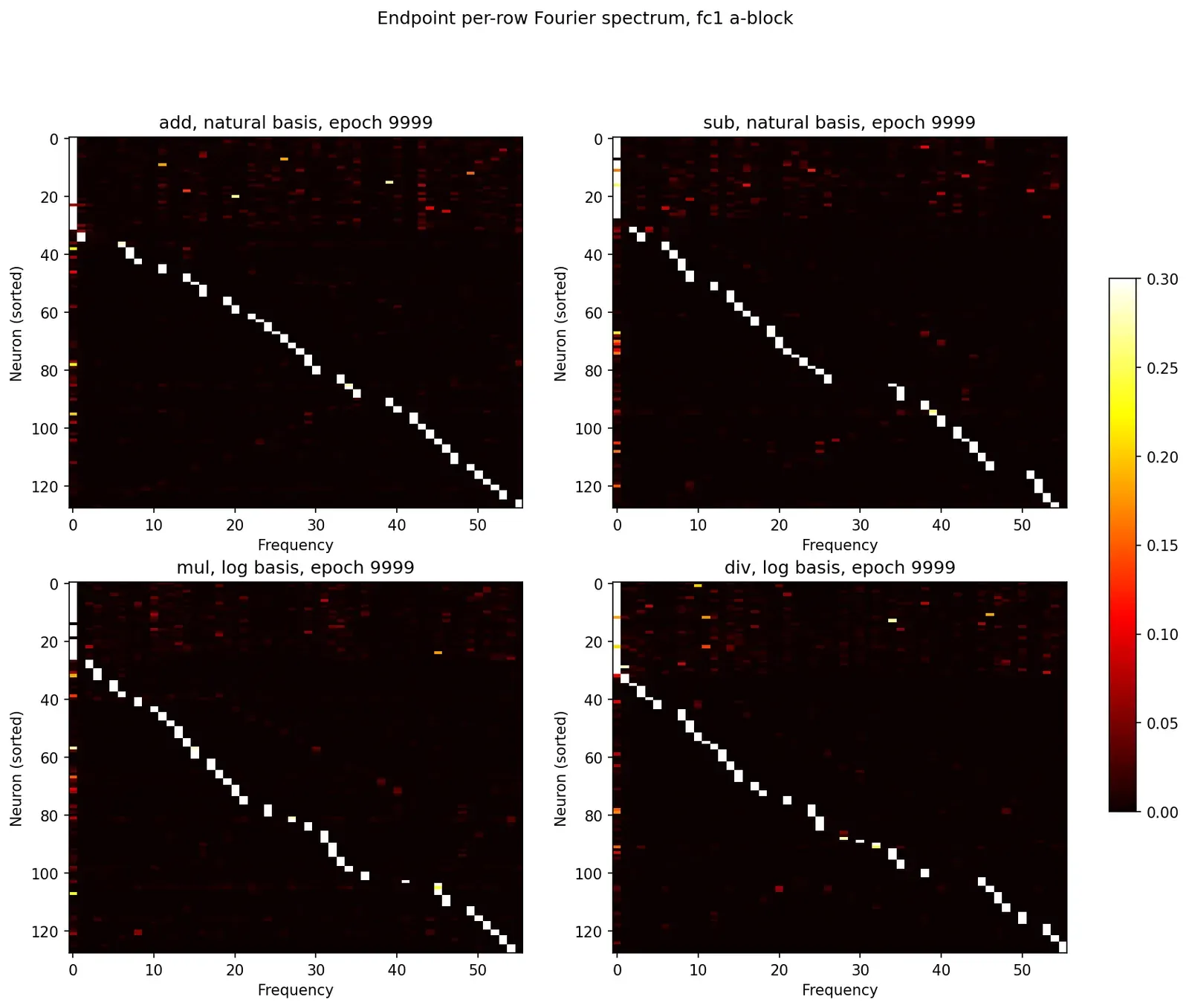
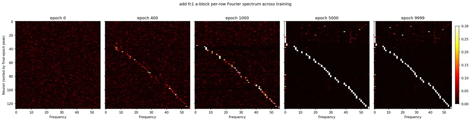
Per-row Fourier spectrum. Where IPR collapses each row to a scalar, the row-wise normalized power spectrum P̃_n,k shows which frequencies are active. We render it as an (N×⌊p/2⌋) heat map, keeping only the first half of the spectrum (informative for real inputs), with rows sorted by their final-snapshot peak frequency so that emerging structure reads as horizontal banding.

Raw weight inspection. For qualitative comparison to (1) we plot W⁽¹⁾_a and W⁽¹⁾_b directly with rows sorted by dominant frequency. A fully grokked solution should display visible sinusoidal striping in each row.

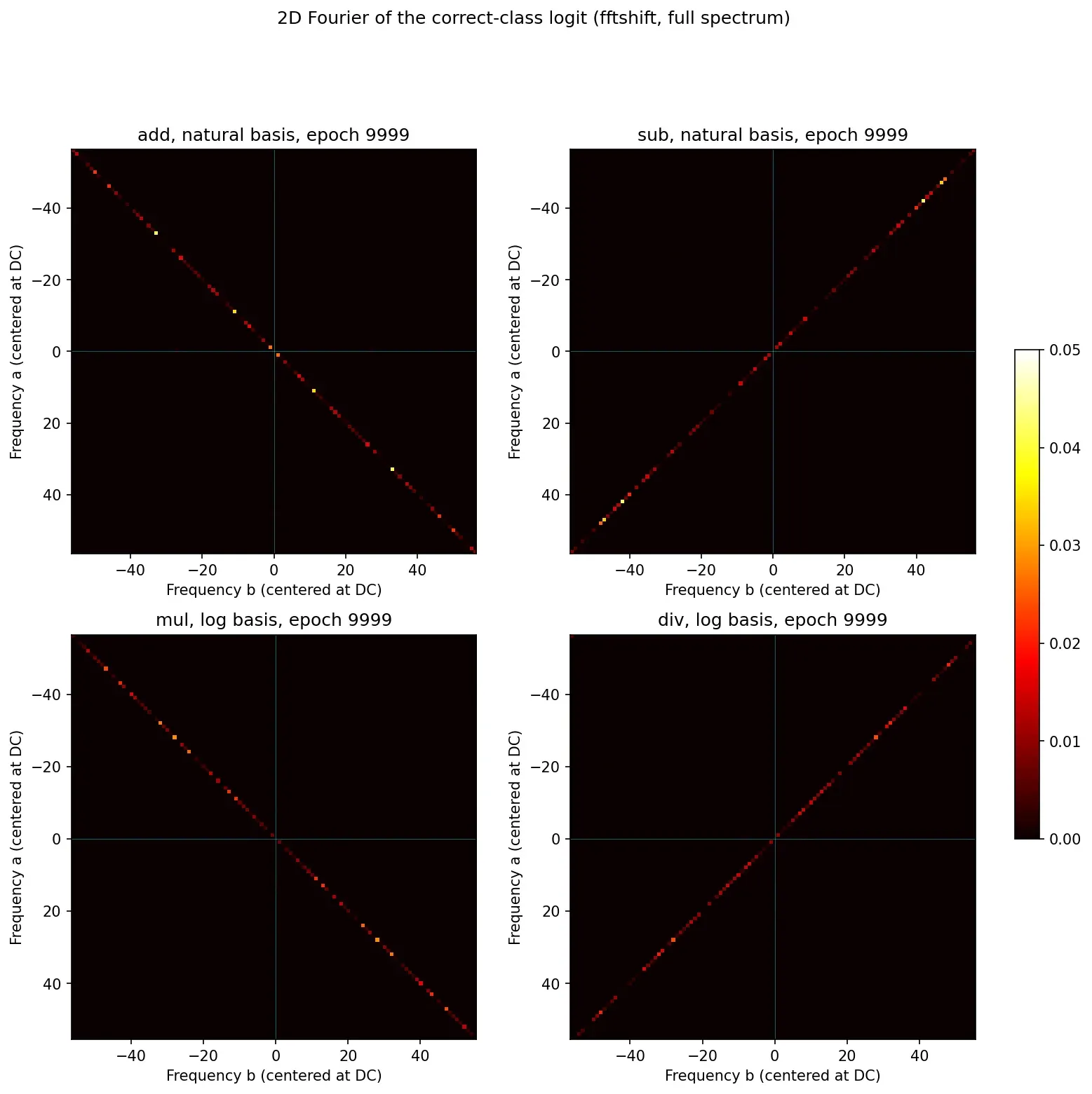
2D Fourier of the correct-class logit. Following [2], we form the matrix M[a, b] = f(e_a, e_b)_{(a⋆b) mod p} of the logit assigned to the correct class for every input pair, and take its 2D FFT. A circuit implementing the trigonometric-identity algorithm of [2] produces sparse peaks in |ℱ_2D[M]|² on the diagonal ω_a=ω_b for additive operations, and on the corresponding diagonal in the log basis for multiplicative operations. This measure is operation-agnostic and end-to-end, complementing the layer-wise IPR.

D. Loss landscape analysis

To complement the spectrum-based view with a geometric one, we project each weight trajectory {(W⁽¹⁾_t, W⁽²⁾_t)} to two dimensions via PCA on the flattened, mean-subtracted snapshots; for both add and mul (seed 0), the top two principal directions explain at least 86% of the trajectory variance. We evaluate train and test MSE on a grid in this plane and plot the resulting log₁₀-loss surfaces with the projected trajectory overlaid. Because PCA selects directions the optimizer was happy to traverse, the resulting surface is biased toward looking like a basin; as a sanity check we also evaluate loss along filter-normalized random directions in the sense of [7].

We trained a 2-layer ReLU MLP on each of the four modular operations across 5 random seeds for 20 runs total, and present the results in roughly the order of the questions posed in §I: that grokking is reliably reproduced (§IV-A), that hidden progress generalizes from transformers to MLPs (§IV-B), that the four trajectories are universal under basis correction (§IV-C), that log-basis structure and Fourier concentration emerge simultaneously rather than sequentially (§IV-D), and that the endpoint weights match the closed-form predictions of [3], [4] (§IV-E).

A. Training dynamics across operations

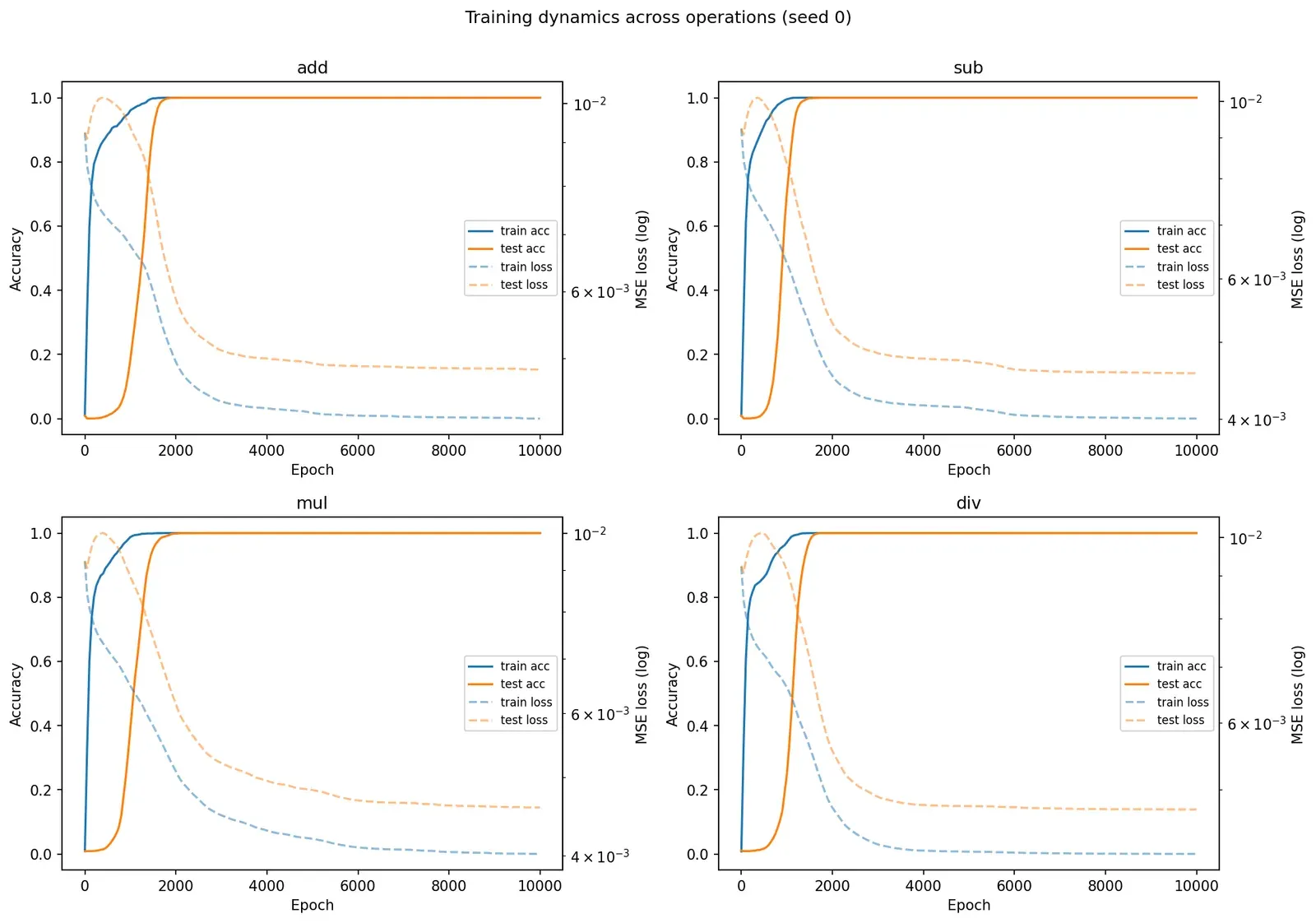
All 20 runs reach 100% test accuracy with the canonical grokking signature, with train accuracy saturating by approximately epoch 250 and test accuracy following only by approximately epoch 1500 (slightly later for multiplication and division). The train and test loss curves of Fig. 1 show the characteristic test-loss bump near the onset of grokking that distinguishes this regime from the comprehension phase of [5]. This confirms our hyperparameter choices place each run inside the grokking phase rather than the comprehension or memorization phases, providing the long memorization plateau in which the progress measures below are evaluated.

B. Hidden progress generalizes to MLPs

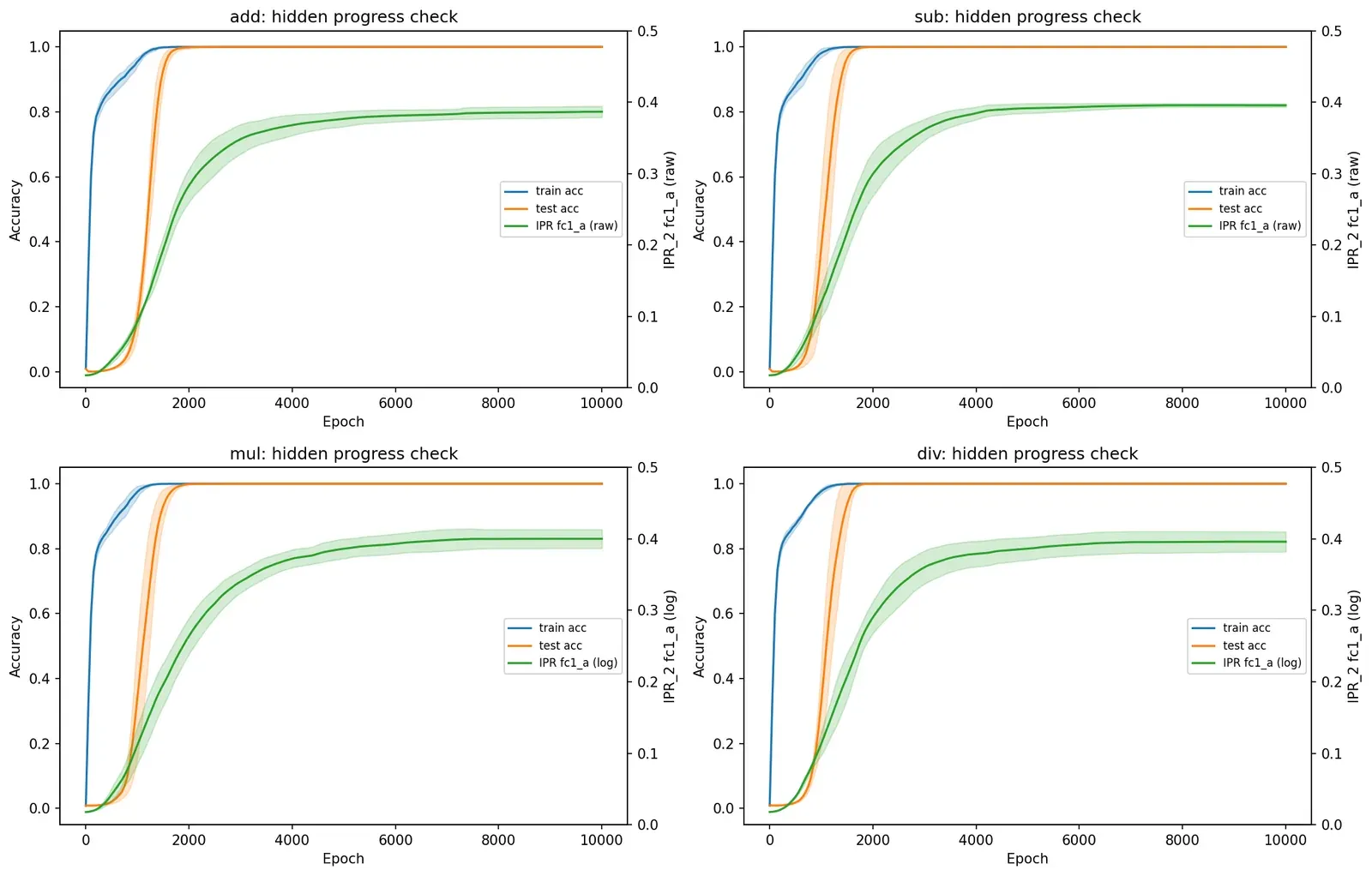
For every operation, the IPR of the first-layer weights climbs smoothly from the random baseline 1/p ≈ 0.009 toward approximately 0.4 during the memorization plateau, well before any movement in test accuracy (Fig. 2). The structural circuit predicted by Eq. (1) therefore forms gradually during the apparent plateau in external metrics, generalizing the hidden-progress finding of [2] from a 1-layer transformer on addition to 2-layer MLPs on all four modular operations. The trajectory is not specific to architecture or operation: it reflects a property of the underlying learning dynamics.

C. A universal trajectory under basis correction

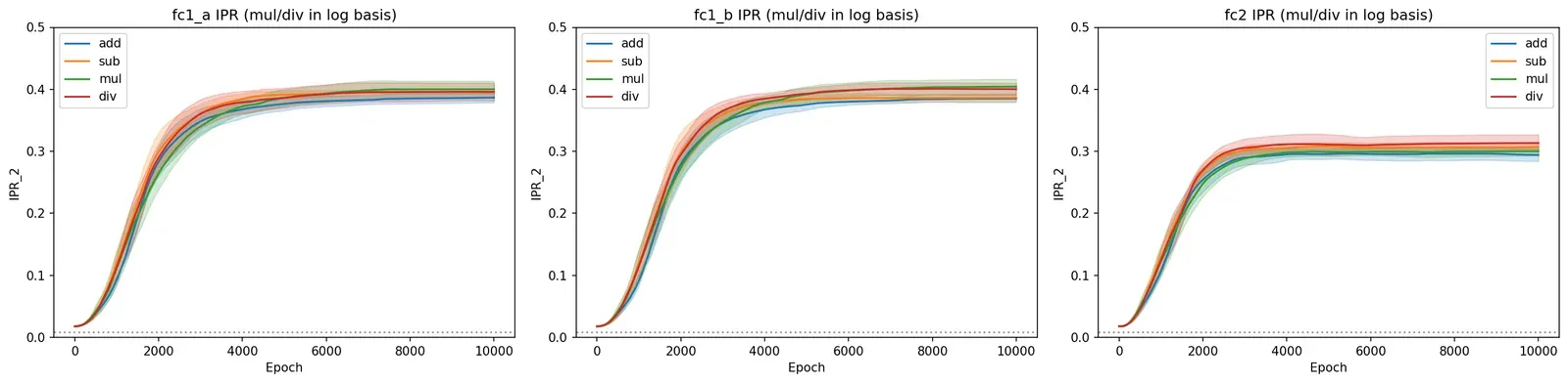
With multiplication and division evaluated in the discrete-log basis introduced in §II-C, the IPR trajectories of all four operations overlap within their seed bands across all three weight blocks W⁽¹⁾_a, W⁽¹⁾_b, and (W⁽²⁾)^⊤ (Fig. 3). Each block rises from the random baseline beginning around epoch 700 and saturates near 0.4 for the first-layer blocks and near 0.3 for the readout, with the four operations indistinguishable up to seed variance. Once the appropriate basis is fixed, the trajectory is universal: the operation-specific aspect of the learning problem is the basis itself, not the dynamics within it. This bridges the endpoint analyses of [3], [4] with the trajectory analysis of [2] into a single picture.

D. Log-basis structure and Fourier concentration emerge simultaneously

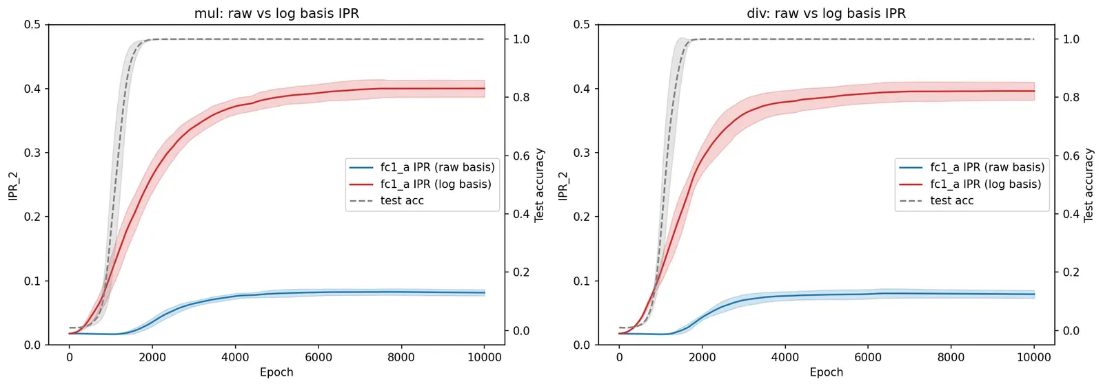
A natural prediction from the structure of Doshi et al.'s closed form is that learning the multiplicative tasks requires two distinct steps: first acquiring the discrete-log permutation that converts multiplication into addition, then concentrating Fourier energy at the resulting frequencies. Fig. 4 refutes this two-stage hypothesis. The log-basis IPR of W⁽¹⁾_a (red) rises in unison with test accuracy (gray) for both multiplication and division, while the raw-basis IPR (blue) saturates at approximately 0.08 throughout training and never approaches the log-basis value. The two structures appear together; we observe no temporal separation between log-basis emergence and Fourier concentration. The network does not first learn a permutation and then sharpen its features against it but instead reaches a solution in which both properties hold jointly.

E. Endpoint weights match the closed form

At the end of training, the per-row Fourier spectra of W⁽¹⁾ in the correct basis show approximately 70–80 of the 128 hidden neurons each locked onto a single frequency, producing the diagonal banding predicted by Eq. (1) (Fig. 5). The remaining neurons sit near DC and are effectively decayed under the weight-decay regularization.

The filmstrip in Fig. 6 shows that this banded structure is not present at initialization and emerges progressively during the memorization plateau, with neurons gradually rather than abruptly committing to specific frequencies as training proceeds.

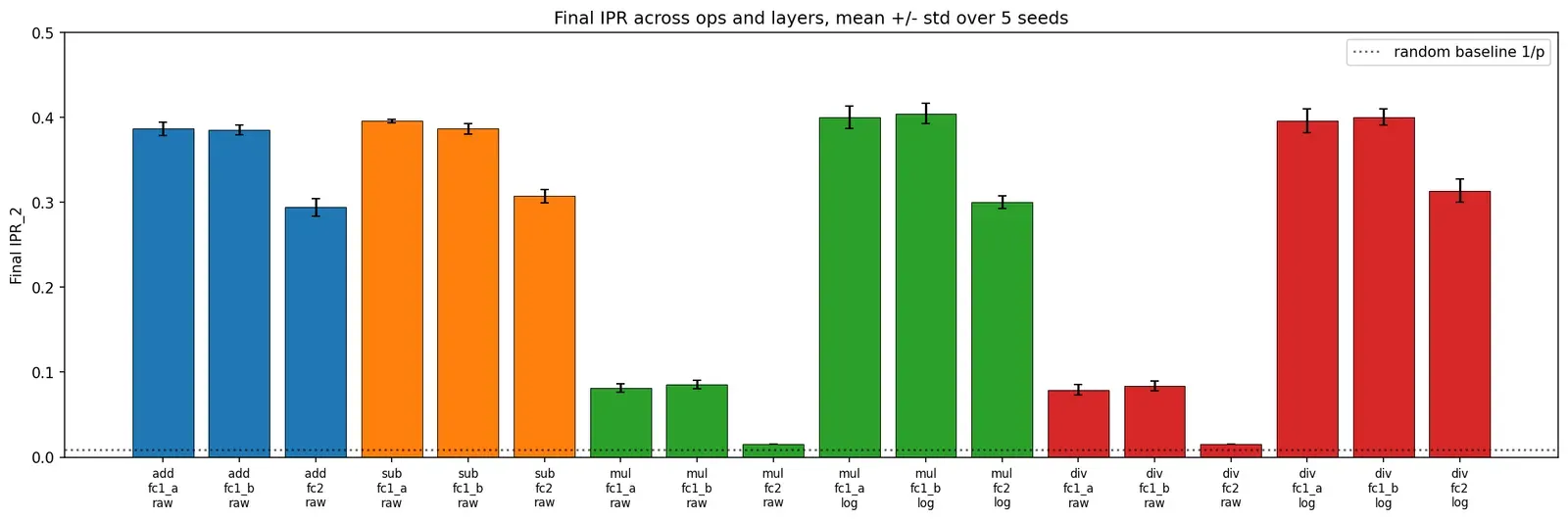
The endpoint IPR values quantify this convergence. In the correct basis, W⁽¹⁾_a and W⁽¹⁾_b reach mean IPR values around 0.40 across all four operations with seed standard deviation below 0.015, and W⁽²⁾ reaches approximately 0.30 (Fig. 7). In the raw basis for multiplication and division, W⁽¹⁾ collapses to approximately 0.08 and W⁽²⁾ to the random baseline, demonstrating that the structure is genuinely basis-specific rather than a property of the raw weight values. The intermediate value of 0.08 is itself informative: the raw-basis weights are not pure noise (which would sit at 1/p≈0.009) and are consistent with weights that encode meaningful structure under a permutation of their indices.

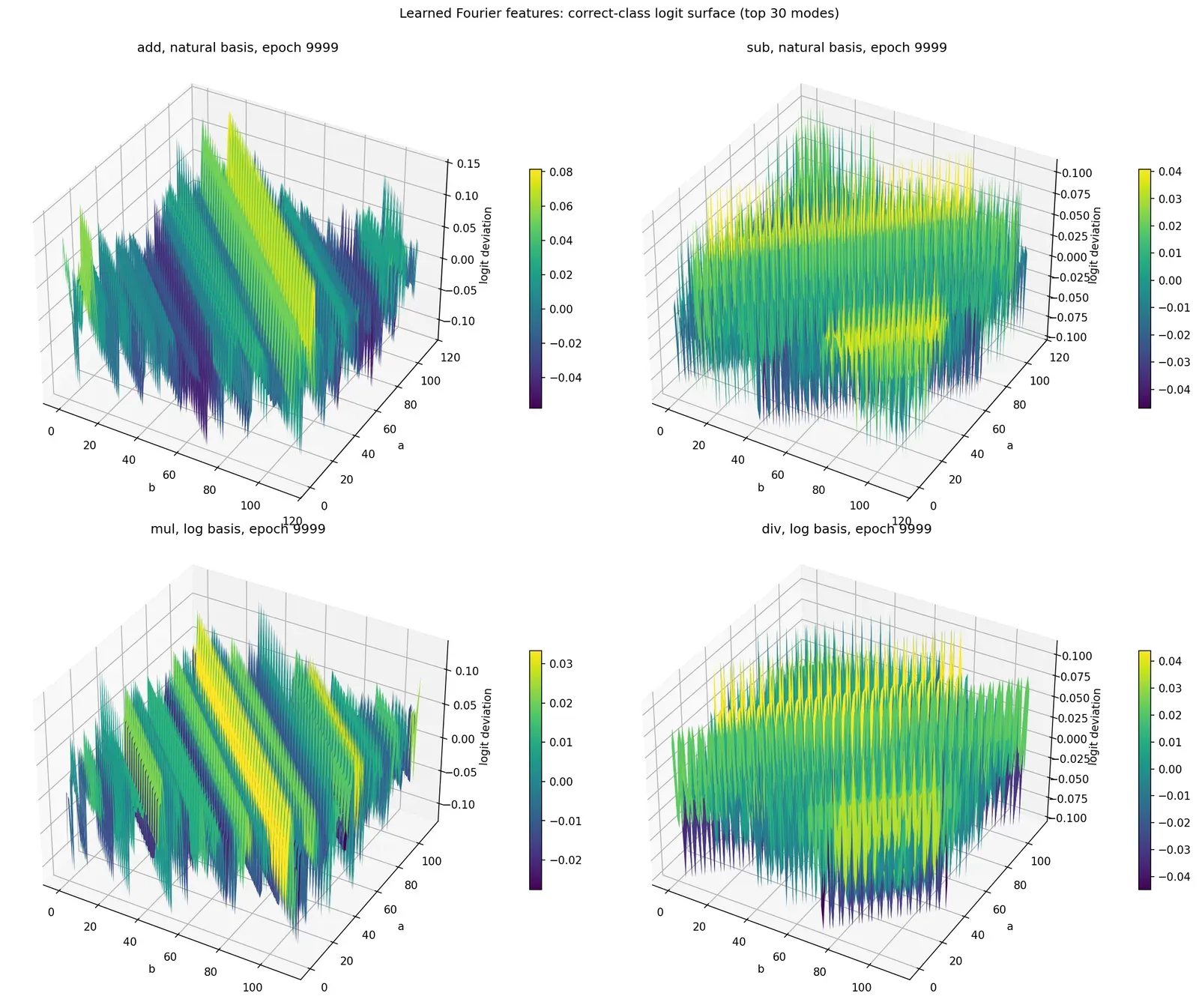
The activation-level view confirms the same picture. Plotting the deviation of the correct-class logit from its mean across all input pairs (Fig. 8) reveals the dominant cosine wave predicted by the trigonometric-identity algorithm of [2], with smaller-amplitude residual modes layered on top.

The 2D Fourier transform of the same correct-class logit grid concentrates power on a sparse diagonal ω_a=ω_b for the additive operations and on the corresponding diagonal in the log basis for the multiplicative ones (Fig. 9), confirming the trigonometric-identity circuit at the level of the network's outputs.

F. Loss landscape geometry

To complement the spectrum-based view with a geometric one, we project the weight trajectory of a representative addition run onto the top two principal components of its weight snapshots, capturing 89% of the trajectory variance, and evaluate the train and test loss on a grid in this plane. The grokked solution sits at the bottom of a clean basin in both train and test surfaces with comparable curvature, consistent with a generalizing rather than overfit minimum. The qualitative geometry is similar for the multiplication run on which we replicated this analysis (not shown).

G. Summary of findings

These results answer the three questions posed in §I. First, the per-row spectra and filmstrip indicate that Fourier modes do not appear in a systematic temporal order; rather, the spectrum sharpens monotonically during the memorization plateau, with neurons gradually committing to specific frequencies as training proceeds. Second, after applying the discrete-log basis correction to multiplication and division, the IPR trajectories of all four operations collapse onto a single curve within seed variance, indicating that the basis is the only operation-specific aspect of the learning problem at the trajectory level. Third, for multiplication and division, the discrete-log basis structure and Fourier concentration emerge simultaneously, refuting the two-stage hypothesis suggested by the structure of the closed-form solution. Together, these findings bridge the endpoint analyses of [3], [4] with the trajectory analysis of [2], extending the latter's hidden-progress framework from a 1-layer transformer on addition to 2-layer MLPs on all four basic modular arithmetic operations.

References

- A. Power, Y. Burda, H. Edwards, I. Babuschkin, and V. Misra, “Grokking: Generalization beyond overfitting on small algorithmic datasets,” in ICLR Workshop on Math. Reasoning in AI, 2022.
- N. Nanda, L. Chan, T. Lieberum, J. Smith, and J. Steinhardt, “Progress measures for grokking via mechanistic interpretability,” in International Conference on Learning Representations (ICLR), 2023.
- A. Gromov, “Grokking modular arithmetic,” 2023.
- D. Doshi, T. He, A. Das, and A. Gromov, “Grokking modular polynomials,” in ICLR 2024 Workshop on Bridging the Gap Between Practice and Theory in Deep Learning, 2024.
- Z. Liu, O. Kitouni, N. Nolte, E. J. Michaud, M. Tegmark, and M. Williams, “Towards understanding grokking: An effective theory of representation learning,” in Advances in Neural Information Processing Systems (NeurIPS), 2022.
- X. Davies, L. Langosco, and D. Krueger, “Unifying grokking and double descent,” in NeurIPS 2022 ML Safety Workshop, 2022.
- H. Li, Z. Xu, G. Taylor, C. Studer, and T. Goldstein, “Visualizing the loss landscape of neural nets,” in Advances in Neural Information Processing Systems (NeurIPS), 2018.